What are the most important patterns in human names?
- 18 minsFinding Patterns in Personal Names (part 1)
Introduction
In this series of blog posts, I am going through a process of finding syntatic patterns of personal names. This is relevant to my “Names” project, in which I was looking at building a flexible model for name classification tasks. However in these blogposts we are only interested in finding the syntatic/linguistic patterns of personal names and do not try to build a working model.
Skill sets
- Basic skills in this series of posts include tree-based models (bagging and boosting), vector-based text modelling and (a bit of) neural networks.
- Most code are written in Python; however I will occasionally move to R in some tasks due to the excellent R package’s ggplot.
Part 1: What are the most important syntatic patterns in names?
In this post, we are trying to follow human instinct while guessing where a person coming from.
-
Normally when I told people my first name,
Hai, most of the time they would say I was from China. Not quite. -
If I told them my middle name, removed for privacy, then they would have another guess, from Korea or China.
-
Finally, when they knew my last name,
Nguyen, 75% of them made a correct prediction
So which features in a name that enable us to correctly guess where a person come from, or even their gender, age, etc?
The first and easy answer would be linguistic/syntatic features.
In this blog post, we will look at the importance of such syntatic features (sub-words) in name classification. We are going to do this by using some extensions of tree bagging models Random Forest and Extremely Randomized Trees to classify the datasets and then using feature importance of each model to see which parterns are more important in classifying names. We also look at a boosting tree model like xgboost to see if there is any difference.
%matplotlib inline

import matplotlib
import matplotlib.pyplot as plt
from __future__ import print_function
import numpy as np
import pandas as pd
from sklearn.model_selection import cross_val_score
Loading the Olympics Data
Firstly we want to load the data and have some initial look. We gonna use a dataset consisting Olympics athletes’ name and countries from the last 2 Olympics Games (2012 and 2016). To try not to make the posts too length, I have collected and cleaned a bit of the dataset so it is ready to use. The original datasets are available here: 2012 and 2016.
names = pd.read_csv('data/fullname_olympics_1216.csv')
names[:10]
| fullname | country | |
|---|---|---|
| 0 | #jesus $garcia | ES |
| 1 | #lam $shin | KR |
| 2 | #aaron $brown | CA |
| 3 | #aaron $cook | MD |
| 4 | #aaron $gate | NZ |
| 5 | #aaron $royle | AU |
| 6 | #aaron $russell | US |
| 7 | #aaron $younger | AU |
| 8 | #aauri #lorena $bokesa | ES |
| 9 | #ababel $yeshaneh | ET |
To remove ambiguity between forenames and surnames, I annotated forenames with prefix # and surnames with prefix $. Now let’s plot the distribution of the names by country (for clarity we only show countries with over 20 names).
plt.rcParams['figure.figsize'] = [20, 8]
names['country'].value_counts()[names['country'].value_counts()>=20].plot.bar()
<matplotlib.axes._subplots.AxesSubplot at 0x7fc893aabc50>
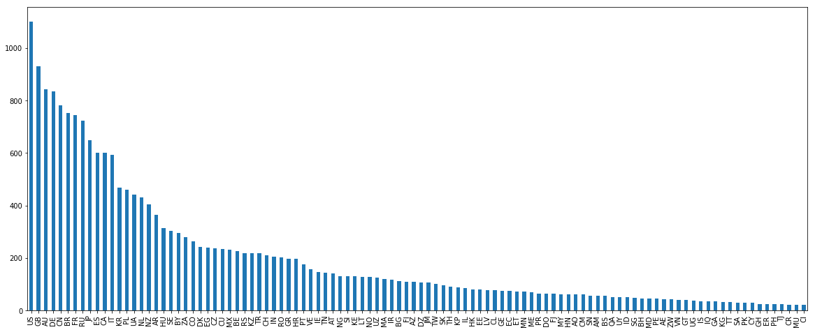
There are many US and AU names in this dataset as the US is among the top sports country. However, a big issue is that they are also a immigration country. Let’s have a look at some US names.
names[names.country=='US'].head(5)
| fullname | country | |
|---|---|---|
| 6 | #aaron $russell | US |
| 12 | #abbey $d'agostino | US |
| 13 | #abbey $weitzeil | US |
| 60 | #abigail $johnston | US |
| 100 | #adeline #maria $gray | US |
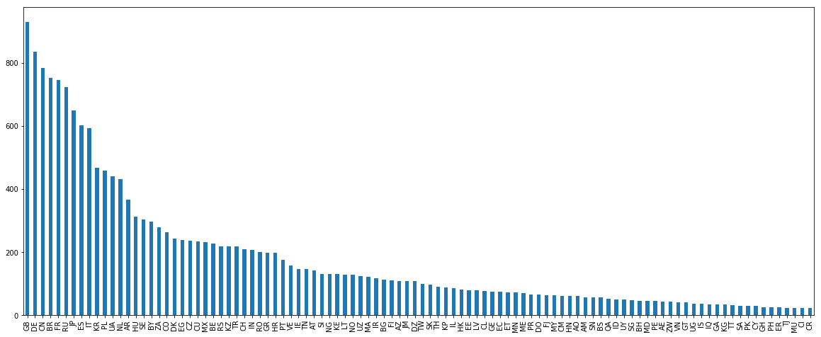
This US group doesn’t look very good. Names like d’agostino or “weitzeil” will bring a lot of noise to our models. So I decided to get rid of it (for now). Sometimes having more doesn’t mean better. We have similar problems in other immigration countries like Canada and New Zealand so I might need to also filter out these countries.
filtered_names = names[~names.country.isin(['CA','US','NZ','AU'])]
print(len(filtered_names['country'].value_counts()[names['country'].value_counts()>=20]))
filtered_names['country'].value_counts()[names['country'].value_counts()>=20].plot.bar()
102


<matplotlib.axes._subplots.AxesSubplot at 0x7fc893c026d8>
filtered_names = filtered_names[filtered_names['country'].isin(filtered_names['country'].value_counts()[filtered_names['country'].value_counts()>=15].index)]
Extracting N-grams Features
To extract n-grams from names, the easiest way is to use sklearn.feature_extraction.text.* packages such as CountVectorizer, HashingVectorizer, TfidfVectorizer… The first two are mainly for count and n-gram features while the last is count features with TF-IDF weights applied to it (TF is term frequency and IDF is the inversed-document frequency weights indicating the importance of a word within a corpus). In this post I used CountVectorizer as it is more intuitive and straight-forward to lookup features. Next we create a vectorizer and feed the names dataframe into it.
To be able to choose the number of ngrams (vocabulary size in memory), let just see how much the vocabulary size changes w.r.t. the size of ngrams. This is quite important as the vocabulary of features in CountVectorizer are stored in memory and having too many sparse but not really necessary features can bring more noise to your models and at the same time occupied unnecessary memory. In theory n-ngram with n characters would take up to (approx) 26^n features, but in practice this number is much smaller. Let’s have a look at this:
from sklearn.feature_extraction.text import *
data = []
for i in range(1,7):
    ngram_vectorizer = CountVectorizer(lowercase=False, analyzer = 'char_wb', ngram_range = (i,i))
    ngram_vectorizer.fit(names['fullname'])
    data.append([len(ngram_vectorizer.vocabulary_),26**i])
print(data)
plt.semilogy(data)
plt.grid(True)
plt.show()
[[35, 26], [791, 676], [8367, 17576], [38506, 456976], [72654, 11881376], [84350, 308915776]]
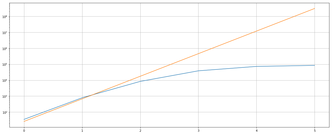
Let’s choose the vocabulary size of 100K (10^5) as this would cover most of the features with n-ngram ranging from 3 to 6 characters since we are intertested in patterns, not performance… In practice I recommend using much lower vocab size as it will make the model more roburst and save your a lot more time. Note that we use the analyzer char_wb to count n-grams of characters and remove unnecessary ngrams in the border of words (with white spaces). I also removed token whose count less than 3 (possibly just typoes).
from sklearn.feature_extraction.text import *
ngram_vectorizer = CountVectorizer(lowercase=False, analyzer = 'char_wb', ngram_range = (3,6),max_features=100000,min_df=3)
ngram_vectorizer.fit(filtered_names['fullname'])
print(len(ngram_vectorizer.get_feature_names()))
ngram_vectorizer.get_feature_names()[:10]
50461


[' #a',
 ' #aa',
 ' #aar',
 ' #aaro',
 ' #ab',
 ' #abb',
 ' #abba',
 ' #abbo',
 ' #abd',
 ' #abda']
Now we only have around 50K patterns left, which is much better. Next let’s try to transform the names into vectors of n-grams. Storing a matrix of 20Kx50K would take a lot of memory (number of cells would be 1 billion); however luckily in sklearn this was stored in a sparse format (a special format that helps to save space and memory when you have many duplicated values likes zeroes or constants).
data =  ngram_vectorizer.transform(filtered_names['fullname'])
label = filtered_names['country']
# since xgboost package doesn't accept string labels, we need to encode them into numeric values
from sklearn.preprocessing import LabelEncoder
le = LabelEncoder()
le = le.fit(label)
encoded_label = le.transform(label)
We need to also transform the labels into number (int) as xgboost classifier doesn’t accept the string labels. In sklearn, you can use LabelEncoder for this task. This is very useful as they can do the inversed mapping by calling inversed_transform to convert from the integer into the string labels.
Building the Models to Find Most Important Patterns
In this section we will build the tree-based models from the sklearn.ensemble package and xgboost in python. We will also look at the most important patterns in each model and see if they are overlapping each other.
Tree-based models
Tree-based learning model is a class of machine learning models utilising decision trees. It could be a single tree or a composition of multiple trees which is also known as an ensemble. The main difference between tree-based ensemble models are whether the trees was build independently (e.g., Random Forest) or one after another (e.g., gradient boosting). Normally for each tree, the algorithm only selects a random sample of the dataset (so called boostrap) and then multiple trees will be combined to get an additive model.
Random Forest
Firstly we gonna try Random Forest and look at the feature importances.
from sklearn.ensemble import *
rf = RandomForestClassifier(n_estimators=100,random_state=42,n_jobs=-1)
rf.fit( data,encoded_label)
RandomForestClassifier(bootstrap=True, class_weight=None, criterion='gini',
            max_depth=None, max_features='auto', max_leaf_nodes=None,
            min_impurity_decrease=0.0, min_impurity_split=None,
            min_samples_leaf=1, min_samples_split=2,
            min_weight_fraction_leaf=0.0, n_estimators=100, n_jobs=-1,
            oob_score=False, random_state=42, verbose=0, warm_start=False)
rf.feature_importances_
array([1.04790809e-03, 1.41188986e-05, 1.46378045e-06, ...,
       0.00000000e+00, 1.03540043e-06, 1.50053925e-07])
sorted_features_idx = np.argsort(rf.feature_importances_)
top_pattern_size = 500
rf_sorted_feature_names = [ngram_vectorizer.get_feature_names()[i] for i in sorted_features_idx[-top_pattern_size:]]
# get top patterns sorted by importance
top_features = list(zip(rf_sorted_feature_names, sorted_features_idx[-top_pattern_size:], np.sort((100*rf.feature_importances_),axis=0)[-top_pattern_size:]))
# print top patterns after removing 1 character pattern
[(feature_name,idx,importance) for (feature_name,idx,importance) in top_features if len(feature_name.replace('#','').replace('$','').strip())>1][-10:]
[('an ', 17793, 0.10845955968255647),
 ('sen', 43988, 0.1095635006092101),
 ('shi', 44195, 0.1186171411838533),
 ('ova', 40078, 0.12612620261085633),
 ('ez ', 26046, 0.13921838947549992),
 ('er ', 25116, 0.16281919553354393),
 ('va ', 48274, 0.1632053337312486),
 ('ic ', 29101, 0.19939663183970113),
 ('ng ', 37022, 0.2004263345017378),
 ('ov ', 40077, 0.20494469651043337)]
Looking good. We would expect something very similar with ExtraTrees.
ee = ExtraTreesClassifier(n_estimators=100,random_state=42,n_jobs=-1)
ee.fit( data,encoded_label)
sorted_features_idx = np.argsort(ee.feature_importances_)
top_pattern_size = 500
ee_sorted_feature_names = [ngram_vectorizer.get_feature_names()[i] for i in sorted_features_idx[-top_pattern_size:]]
# get top patterns sorted by importance
top_features = list(zip(ee_sorted_feature_names, sorted_features_idx[-top_pattern_size:], np.sort((100*ee.feature_importances_),axis=0)[-top_pattern_size:]))
# print top patterns after removing noise (1 character pattern)
[(feature_name,idx,importance) for (feature_name,idx,importance) in top_features if len(feature_name.replace('#','').replace('$','').strip())>1][-10:]
[('ez ', 26046, 0.10765161976804602),
 ('na ', 36311, 0.10796082306967256),
 ('vic ', 48607, 0.10807446223769633),
 ('an ', 17793, 0.11214521989802909),
 ('sen ', 43989, 0.12211872837731705),
 ('va ', 48274, 0.1273201187308604),
 ('ng ', 37022, 0.13157069547920763),
 ('er ', 25116, 0.13579010957546528),
 ('ov ', 40077, 0.1591217190628161),
 ('ic ', 29101, 0.17477829732484954)]
print('#patterns in intersection',len(list(set(rf_sorted_feature_names)&set(ee_sorted_feature_names))))
print('#patterns in rf model only',len(list(set(rf_sorted_feature_names) - set(ee_sorted_feature_names))))
## print set difference features
# print(pd.DataFrame(list(set(rf_sorted_feature_names) - set(ee_sorted_feature_names))))
print('#patterns in ee model only',len(list(set(ee_sorted_feature_names) - set(rf_sorted_feature_names))))
## print set difference features
# print(pd.DataFrame(list(set(ee_sorted_feature_names) - set(rf_sorted_feature_names))))
#patterns in intersection 441
#patterns in rf model only 59
#patterns in ee model only 59
90% of the top 500 patterns of the first 2 models are overlapping. Now let’s try a completely different model, xgboost that ensembles the trees in a boosting manner instead of boostrap samples and aggregate them like in bagging. Note that in RF and EE models, we didn’t limit the max as we try to build complex trees and average them out so that overfitting can be avoid. In xgboost, we use smaller trees (can even with depth of 2 or 3), but many of them to refine the model in an incremental way.
from xgboost import XGBClassifier
xgb = XGBClassifier(n_estimators = 200, max_depth=8,nthread =22,objective='multi:softmax')
xgb.fit( data,encoded_label)
sorted_features_idx = np.argsort(xgb.feature_importances_)
top_pattern_size = 500
xgb_sorted_feature_names = [ngram_vectorizer.get_feature_names()[i] for i in sorted_features_idx[-top_pattern_size:]]
# get top patterns sorted by importance
top_features = list(zip(xgb_sorted_feature_names, sorted_features_idx[-top_pattern_size:], np.sort((100*xgb.feature_importances_),axis=0)[-top_pattern_size:]))
# print top patterns after removing noise (1 character pattern)
[(feature_name,idx,importance) for (feature_name,idx,importance) in top_features if len(feature_name.replace('#','').replace('$','').strip())>1][-10:]
[('ne ', 36853, 0.41213962),
 ('in ', 30169, 0.4258885),
 ('en ', 24662, 0.42818004),
 ('el ', 24248, 0.45109484),
 ('ia ', 28854, 0.514929),
 ('er ', 25116, 0.5201667),
 ('on ', 39021, 0.5362071),
 ('ng ', 37022, 0.57188874),
 ('na ', 36311, 0.795472),
 ('an ', 17793, 1.1467237)]
print('#patterns in xgb and rf intersection',len(list(set(rf_sorted_feature_names)&set(xgb_sorted_feature_names))))
print('#patterns in rf model only',len(list(set(rf_sorted_feature_names) - set(xgb_sorted_feature_names))))
# print(pd.DataFrame(list(set(rf_sorted_feature_names) - set(xgb_sorted_feature_names))))
print('#patterns in xgb model only',len(list(set(xgb_sorted_feature_names) - set(rf_sorted_feature_names))))
# print(pd.DataFrame(list(set(xgb_sorted_feature_names) - set(rf_sorted_feature_names))))
#patterns in xgb and rf intersection 289
#patterns in rf model only 211
#patterns in xgb model only 211
As we can see, RF and EE models are very similar in terms of feature importance with around 90% of top 500 features overlapped. RF and XGB only have 60% of the top 500 features overlapped. Here are major observations from the top features.
- Most important (at least top-10) features are suffixes of a name (can be either surname or forename):
an,ezfor Hispanic names,ovfor Russian names,vicfor Balkan,senfor Dannish names, etc. - Prefixes are much more rare, but seem to be important signals too.
$al,$ch,$zh, are common prefixes for Arabic, German, and Chinese surnames. - Important patterns in XGB are in average shorter than ones in Random Forest and ExtraTrees. It looks like XGB looks at more dominant patterns and less randomised than RF and EE.
- Whole names themselves in top patterns are
#vanand$kim, all of which are popular names in Dutch, Vietnamese and Korea.
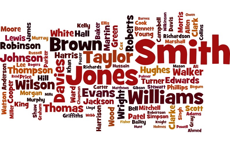
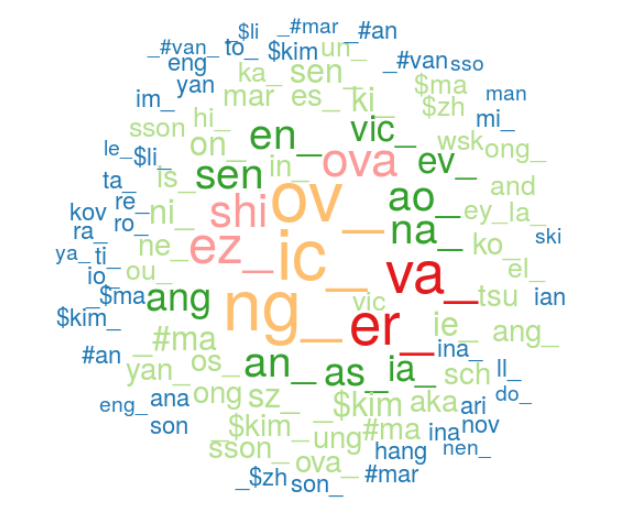
Visualising Top Features
A blogpost should always end with a good visualisation. Here I visualise the top 100 n-grams in terms of importance for the name-based nationality classification task. To keep thing simple I used R’s wordcloud package to produce this plot. We can easily see that most important features are suffixes, although quite a few prefixes of forenames appeared on the top 100.
library(data.table)
top_100_rf_features = fread('~/working/data-fun/blogs/name-patterns/data/rf_top100_features.csv')
top_100_rf_features$V3 <- round(as.numeric(top_100_rf_features$V3)*100)
library(RColorBrewer)
library(wordcloud)
wordcloud(words=top_100_rf_features$V1, freq=top_100_rf_features$V3,min.freq=1,rot.per = 0,random.order = F,random.color = F,colors = brewer.pal(7, "Paired"))
Summary
In this blog post, we’ve gone through the steps to find the most important patterns for the name-based nationality prediction task. In particular, we have:
- loaded the dataset and view some descriptive stats,
- vectorized the full names into a one-hot vector using
sklearn’s feature extraction, - created 3 tree-based models and look at most important patterns. We’ve also looked at overlapping between top patterns among the models:
- Random Forest
- ExtraTrees (Extremely Randomised Trees)
- XGBoost
In the next blog post, we will try to look at which features are important for a specific country, such as the UK or China.

Hai Nguyen
Data Scientist working at the University of Liverpool